My first Python tutorial using Overture data - comparing its building footprint coverage to OSM. First tests show that its coverage is slightly better - even in densely populated, central areas. More comparisons are coming soon!
1. Imports, setting up, data sources, data preparation
import osmnx as ox
import geopandas as gpd
from shapely.geometry import Polygon
import requests
import matplotlib.pyplot as plt
import os
import warnings
warnings.filterwarnings('ignore')

c1 = "#4DFFFD"
c2 = "#ff6ec7"

admin = ox.geocode_to_gdf('5th District, Budapest')
admin.plot()
2. Downloading the data
# Extract the bounding box from the GeoDataFrame
minx, miny, maxx, maxy = admin.total_bounds  # Get bounding box
bbox = f"{minx},{miny},{maxx},{maxy}"       # Format as a string

# Download data from Overture Maps
output_file_overture = "overture_budapest_district5_buildings.geojson"

os.system(f"overturemaps download --bbox={bbox} --type=building  -f geojson --output={output_file_overture}")

overture_buildings = gpd.read_file(output_file_overture)

# Create a bounding box polygon for OSM query
polygon = ox.utils_geo.bbox_to_poly(miny, maxy, minx, maxx)

# Download building data from the same area from OSM
osm_buildings = ox.features_from_polygon(polygon, tags={"building": True})
print(f"OpenStreetMap data loaded. Number of buildings: {len(osm_buildings)}")
3. Creatin the map
f, ax = plt.subplots(1,2,figsize=(7,9))


osm_buildings.plot(ax=ax[0], color = c1)
overture_buildings.plot(ax=ax[0], color = c1, alpha = 0.5)

overture_buildings.plot(ax=ax[1], color = c2, edgecolor = c2, linewidth = 1)
osm_buildings.plot(ax=ax[1], color = 'k')#, alpha = 0.5)


for aax in ax:
    aax.axis('off')

ax[1].set_title('Overture - OSM', fontsize=16, pad=10, color="white")
ax[0].set_title('Overture + OSM', fontsize=16, pad=10, color="white")


f.patch.set_facecolor('black')
plt.tight_layout()
plt.savefig('DAY29.png', dpi = 200, facecolor = 'k')


