Lego Elevation Map

How to turn vector elevation lines into a grid — and build it from Lego

Vector and raster data are the two main types of spatial data structures. Vector data is great for storing exact locations and shapes, such as points, lines, and polygons. In contrast, raster data models spatial features using a grid of pixels, each storing particular values. Different data sources and applications yield different data structures; however, when conducting advanced spatial analytics, we often need to make these two different types meet. In this article, I will give an example of that — how to turn vector data, in this case, elevation lines, into a raster of grid cells. Additionally, I show how this can be visualized by matching each raster grid cell to a small Lego brick.

Data

As a data source, I used the open data provided by the Budapest Open Data Atlas containing the elevation layers of the city. After downloading the spatial data file, let’s have a look at it using GeoPandas:

import geopandas as gpd

gdf = gpd.read_file('bpelev.json')

print(len(gdf))
gdf.head(5)

The output of this cell:

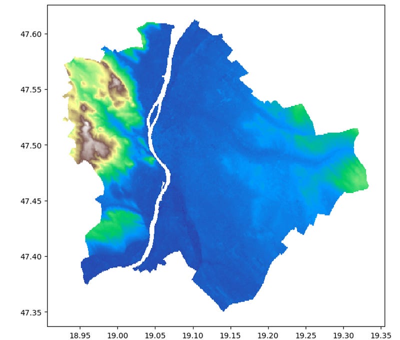
Now, let’s also take a visual look at what these polygons look like. To make an appropriate map from this data, let’s use the ‘terrain’ colormap of Matplotlib.

import matplotlib.pyplot as plt

f, ax = plt.subplots(1,1,figsize = (8,8))
gdf.plot(column = 'DN', ax=ax, cmap = 'terrain')

The resulting visual:

Create a square grid

Now that we had a quick look at the vector data part let’s move towards rasterizing it. First, let’s get a plain map of the administrative boundaries of Budapest from OSM using the OSMnx library:

#Import all the libraries we use
import osmnx as ox  

# Download the administrative boundary of Budapest
admin_city = ox.geocode_to_gdf('Budapest')
admin_city.plot()

The result of this code block:

And now, let’s create a function that splits this polygon into a grid with a given number of cells. Then, also visualize the result with an example splitting resolution:

# Import GeoPandas for geospatial data handling
from shapely.geometry import box 

# Create the grid polygons
def create_grid(minx, miny, maxx, maxy, num_cells_x, num_cells_y):
    grid_polygons = []
    cell_width = (maxx - minx) / num_cells_x
    cell_height = (maxy - miny) / num_cells_y

    for i in range(num_cells_x):
        for j in range(num_cells_y):
            x = minx + i * cell_width
            y = miny + j * cell_height
            grid_polygons.append(box(x, y, x + cell_width, y + cell_height))
    
    return grid_polygons

# Extract the bounding box of Germany from the GeoDataFrame
gdf_example = admin_city
gdf_example.crs = 4326
bounds = gdf_example.bounds

minx = bounds.minx.values[0]
miny = bounds.miny.values[0]
maxx = bounds.maxx.values[0]
maxy = bounds.maxy.values[0]

# Create a 10x10 grid within the bounding box of Germany
grid_polygons = create_grid(minx, miny, maxx, maxy, 22, 22)
gdf_grid = gpd.GeoDataFrame(grid_polygons, columns=['geometry'])
gdf_grid.crs = 4326

# Visualize the grid overlaid on the map of Germany
f, ax = plt.subplots(1, 1, figsize=(8, 8))
gdf_example.plot(ax=ax, color='none', edgecolor='k', linewidth=3)
gdf_grid.plot(ax=ax, edgecolor='w', alpha=0.5)
ax.axis('off')
plt.show()

The map of Budapest and a 22x22 grid mapped onto it:

Map the elevation values into the grid

Now we have both the vector and the raster part — it’s time to make these two meet! First, using spatial join, I determine the overlaps between the polygons of the raster grid cells and the elevation lines e the overlaps between the two. This will result in a square grid polygon where each grid cell has one single value — the mean value of corresponding elevation levels. 

# Perform spatial join to find grid cells that contain the polygons
joined = gpd.sjoin(gdf, gdf_grid, how="left", op="within")

# Aggregate the DN values by the grid cell index
aggregated = joined.groupby('index_right').agg({'DN': 'mean'}).reset_index()

# Merge the aggregated DN values back to the grid cells
gdf_grid['DN'] = gdf_grid.index.to_series().map(aggregated.set_index('index_right')['DN'])
gdf_grid.head()

As my final goal is not just to visualize the elevation map but to do that with Lego bricks, I had to do some scaling to make sure that I have a certain number of discreet elevation levels that I can match with Lego bricks of different colors. While for spatial analytics projects, this step might not be necessary, depending on the final use case, for a fun exercise, this is great.

import numpy as np
import math

gdf_grid['log'] = [math.log(x+1) for x in gdf_grid.DN.to_list()]
values = gdf_grid.log.to_list()
val_min = gdf_grid.log.min()
values = [round(24*((v / val_min)-1))  if not np.isnan(v) else v for v in values]
gdf_grid['height_level'] = values #[v if v<8 else 7 for v in values]
gdf_grid['height_level'] = gdf_grid['height_level'].replace(8, 7)
gdf_grid['height_level'] = gdf_grid['height_level'].replace(7, 6)

print(gdf_grid.height_level.min())
print(gdf_grid.height_level.max())

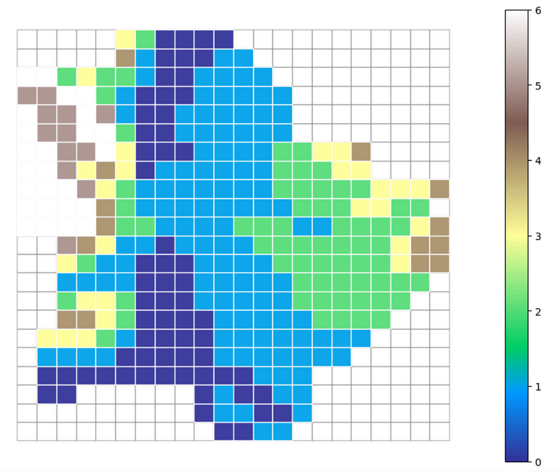
After scaling, all I had left was to discrete elevation grid:

# Visualize the grid overlaid on the map of Germany
f, ax = plt.subplots(1, 1, figsize=(12, 8))

gdf_grid.plot(ax=ax, color = 'w', edgecolor='grey', alpha=0.5)

gdf_grid.plot(ax=ax, column = 'height_level', edgecolor='w', cmap = 'terrain', alpha=0.95, legend = True)

ax.axis('off')
plt.show()