Roadnetworks - A Map with a Plotter

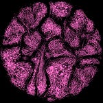
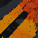
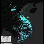
A few years ago, I visited the dataviz workshop/lab of Mihály Minkó and his team and got to learn about their awesome 2d plotter directly driven from Python - and how it is able to visualize networks and maps - and even road networks! Enjoy the footage.

Road networks are beautiful bird-eye view representations of cities.However, their importance reaches far beyond eye candies used as wallpapers. In fact, for the trained urbanist eyes, the visual structure of a city’s road network already hints at lots of information about the masterplan (if there was any) and the possible paths of development a city took, as well as the potential pitfalls and problems currently, or in the near future could affect the city. These can range from public and private transportation planning to the improvement of green infrastructure and the accessibility of services and amenities.

In this article, I introduce you to the first step of this process by using the OSMnx library to download various global cities road networks.

All images were created by the author.

Prototyping the road network visualization process

Let’s start with something simple and quick to process, for instance, a smaller ity district. As an example, I use downtown, District 5, in Budapest.

First, using OSMnx, I download the admin boundaries of the city, and then use the graph_from_polygon command to download the road network within that polygon. As the plotted admin boundaries of this target area shows, it is one single polygon — now we just note this, but later on, we will see that this can make generalization for any administrative area a bit more tricky.

Once we have the road network stored in a graph object, we can check the number of nodes and edges (intersections and road segments) and turn it into two GeoDataFrames: one containing all the nodes and the other containing all the edges.Let’s also plot them separately to have a quick view of these two components.

# import osmnx
import osmnx as ox
city  = '5th District, Budapest, Hungary'

# download and plot the admin boundaries of the target area
admin = ox.geocode_to_gdf(city)
display(admin)
admin.plot()

# Download the road network
G = ox.graph_from_polygon(admin.geometry.to_list()[0])

print('Number of intersections: ', G.number_of_nodes())
print('Number of road segments: ', G.number_of_edges())

# turning the graph into geodataframes
nodes, edges = ox.graph_to_gdfs(G)

Results:

# plotting the two GeoDataFrames extracted from the road network graph
import matplotlib.pyplot as plt
f, ax = plt.subplots(1,2,figsize = (12,5))

nodes.plot(ax = ax[0], color = 'k', markersize = 5)
edges.plot(ax = ax[1], color = 'k', linewidth = 1)

plt.tight_layout()

Visualizing multiple global cities

Now, let’s rip the previous section into pieces and turn it into a more general pipeline for downloading, processing, and visualizing a list of global cities.

Downloading the admin boundaries

Let’s define the list of cities and plot their admin boundaries obtained from OpenStreetMap using OSMnx.

cities = ['Tokyo, Japan', 
          'Delhi, India', 
          'Barcelona, Spain', 
          'Dhaka, Bangladesh', 
          'Sao Paulo, Brazil',
          'Budapest, Hungary']

f, ax = plt.subplots(2,3,figsize=(15,8))
indicies = [(i, j) for i in range(2) for j in range(3)]

for idx, city in enumerate(cities):
    bx = ax[indicies[idx]]
    admin = ox.geocode_to_gdf(city)
    admin.plot(ax=bx)
    bx.set_title(city)

Except for Tokyo, it looks like they all are placed a single well-defined area. That is one problematic city out of six, so let’s take a closer look and clean up the case of Tokyo.

Cleaning up Tokyo

First, let’s create a larger image of the data acquired for Tokyo and visually observe it while also displaying the GeoDataFrame. Note: this will be an example of very practical, boring, yet realistic data cleaning.

city = 'Tokyo, Japan'
  
f, ax = plt.subplots(1,1,figsize=(10,10))
admin = ox.geocode_to_gdf(city)
display(admin)
admin.plot(ax=ax)

Based on the displayed GeoDataFrame, it seems that we have one single record with a multipolygon in it. Additionally, the visuals hint that there are lots of point-like geometries packed into the multi polygon, and only one looks more like an administrative area up north. Let’s see how we can get it algorithmically.

First, let’s explode the multipolygon and plot separately:

import geopandas as gpd

admin_exp = admin.explode('geometry')

f, ax = plt.subplots(4,5,figsize=(15,8))
indicies = [(i, j) for i in range(4) for j in range(5)]

for idx in range(len(admin_exp)):
    bx = ax[indicies[idx]]
    admin_exp_segment = gpd.GeoDataFrame(admin_exp.iloc[idx]).T
    admin_exp_segment.geometry = admin_exp_segment['geometry']
    admin_exp_segment.plot(ax=bx)
    bx.set_title(idx)

Now, I am looking for an algorithmic way to differentiate geometry #2 from the rest, which looks very much like Tokyo. By the way, most of the other geometries look like points buffered to become circles, with a few building-footprint-looking elements there.

The theoretical hint I will use to capture the city is going to be the area — perimeter ratio. Since administrative areas tend to have very detailed, fractal-like boundary lines, as opposed to the smooth boundaries of the other polygons we have, I hope that this indicator, together with a filter on sizes, will help.

Namely, first, I compute the area and length of each geometry. Then, I compute their area , which should be higher and more fractal-like, like the boundary lines. Additionally, I drop the really tiny geometries and then sort the resulting table — which, fortunately, and also somewhat expectedly, is topped by geometry #2.

# import pandas
import pandas as pd

# compute areas and area_length indicies
areas = []
lengths = []

for idx in range(len(admin_exp)):
    admin_exp.iloc[idx]
    areas.append(admin_exp.iloc[idx].geometry.area)
    lengths.append(admin_exp.iloc[idx].geometry.length )
   
# leets pack the geometry area and length values into a DataFrame
df_tokyo = pd.DataFrame({'geometry_index' : range(len(admin_exp)),
                          'areas' : areas,
                          'lengths' : lengths
                         })

# let's compute the area-length ratios,
df_tokyo['areas_length'] = df_tokyo['areas'] / df_tokyo['lengths']

# let's filter out the tiny geometries
df_tokyo = df_tokyo[df_tokyo.areas>0.0001]

# sort the results
df_tokyo.sort_values(by = 'areas_length')

The resulting table:

Final admin boundaries

Now that we have a clean-up receipt for Tokyo, let’s download and plot all city admin boundaries again. Also, let’s store them in a dictionary for the next sections.

f, ax = plt.subplots(2,3,figsize=(15,8))

cities_admins = {}

for idx, city in enumerate(cities):
    bx = ax[indicies[idx]]
    admin = ox.geocode_to_gdf(city)
    if 'Tokyo' in city:
        admin_exp = admin.explode('geometry')
        admin = gpd.GeoDataFrame(admin_exp.iloc[2]).T #,
        admin.geometry = admin['geometry']
    admin.plot(ax=bx)
    bx.set_title(city)
    cities_admins[city] = admin

Visualizing a series of global cities’ road networks

First, let’s download the edge list of all cities and store them in a dictionary. For the sake of simplicity (having a smaller, easier-to-process network), I set the network type to ‘drive’, so now we will only download road networks available for cars. To get all road segments, just drop this input parameter. You can also try other parameter values, such as ‘walk’ or ‘bike’.

city_edges = {}

for city, admin in cities_admins.items():
    G = ox.graph_from_polygon(admin.geometry.to_list()[0], network_type = 'drive')
    nodes, edges = ox.graph_to_gdfs(G)
    print(city, 'number of nodes: ', len(nodes), '   number of edges: ', len(edges))
    city_edges[city] = edges 

Then, let’s create a drafty plot of them:

f, ax = plt.subplots(2,3,figsize=(15,8))

city_edges = {}
for idx, (city, edges) in enumerate(cities_edges.items()):
    bx = ax[indicies[idx]]
    edges.plot(ax = bx, linewidth = 0.3)
    bx.axis('off')

Now, let’s create a color palette. In this case, I used ChatGPT to get a list of neon colors and matching backgrounds. Finally, let’s use this color palette to visualize the road networks of all six cities as follows:

# define the colors
color_palette = [{"Neon": "#ff0099",  "Background": "#2e002e"},
                 {"Neon": "#00ff00",  "Background": "#003300"},
                 {"Neon": "#00ccff",  "Background": "#002233"},
                 {"Neon": "#ffff00",  "Background": "#333300"},
                 {"Neon": "#ff6600",  "Background": "#331a00"},
                 {"Neon": "#ff00ff",  "Background": "#330033"}
]


# visualize networks
for idx, (city, edges) in enumerate(city_edges.items()):   
    
    # set the plot paramts
    neon = color_palette[idx]['Neon']
    color_bcg  = color_palette[idx]['Background']
    width = 0.5

    # do the plot
    f, ax = plt.subplots(1,1,figsize=(12,12))
    edges.plot(ax = ax, color = neon, linewidth = width, alpha = 0.9)
    ax.set_facecolor(color_bcg)

    # get rid of the ticks
    for xlabel_i in ax.get_xticklabels(): xlabel_i.set_visible(False)
    for ylabel_i in ax.get_yticklabels(): ylabel_i.set_visible(False)
    for tick in ax.get_xticklines(): tick.set_visible(False)
    for tick in ax.get_yticklines(): tick.set_visible(False)

    # add the title
    ymin, ymax = plt.ylim()
    extension = 0.1 * (ymax - ymin)
    ax.set_ylim(ymin, ymax + extension)
    ax.set_title(city, fontsize = 20, color = neon, y = 0.9)

Conclusion

In this piece, we reviewed how to download and visualize road networks of various global cities, which are not only useful ways of representing urban environments but also serve as a basis for various analytical exercises in different domains of urban planning. Additionally, via the example of Tokyo, we did a de-tour of those waters, which tutorials tend to neglect — the ugly and painful part of case-by-case data cleaning to arrive at a generic pipeline easy-to-adopt to a multitude of cities.

In case you would like to read more on spatial networks and further advance your geospatial Python skills, check out my brand new book, Geospatial Data Science Essentials — 101 Practical Python Tips and Tricks!